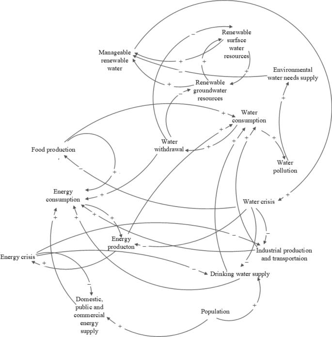
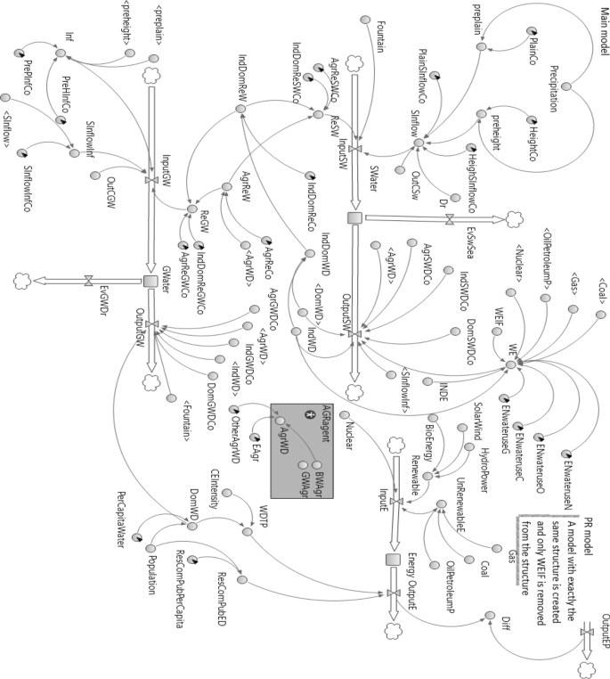
The effect of reducing per capita water and energy uses on renewable water resources in the water, food and energy nexus

This work formulates a general framework of the WFE Nexus at the national level, which includes all pertinent interactions between water, food, and energy sources and demands. Figure 1 depicts the feedbacks involving resource availability and consumption. The causal loops of the developed model for national-scale assessment are shown in Fig. 2. The model depicted in Fig. 2 proposes reducing consumption to reduce the water crisis to the extent possible. By reducing water use and pollution the environmental water requirement can be reduced, thus alleviating the water crisis. This paper’s objective is sustainable management by reducing per capita water use (in the residential section) and per capita energy use (in the domestic, public, and commercial section). The WFE nexus is modeled as a dynamic system for demand management applied to the stocks of energy, surface water, and groundwater resources to calculate their input and output rates (flows) at the national level while providing for environmental flow requirements (Fig. 3). The national modeling approach is of the lumped type, meaning that inputs and outputs to the stocks of water and energy represent totals over an entire country (in the case study, Iran); therefore, the models does not consider intra-country regional variations. The units of water resources and energy resources are expressed in cubic meters and MWh, respectively.

Table of Contents

Balance of water resources

The study of water exchanges in a country is based on the law of conservation of matter. The following sections present calculations pertinent to the annual balance of surface and groundwater resources.

Surface water resources

The national runoff generated in a country’s high-elevation areas (or high terrain) and low-elevation areas (plains) is quantified with the following equations:

$$preheight_t=HeightCo\times Precipitation_t$$

(1)

in which $preheight_t$ = volume of precipitation that falls in high-elevation areas during period t, $HeightCo$ = the percentage of total precipitation that falls in high-elevation areas, and $Precipitation_t$ = volume of precipitation during period t.

$$preplain_t=PlainCo\times Precipitation_t$$

(2)

in which $preplain_t$ = volume of precipitation that falls in the plains during period t, and $PlainCo$ = the percentage of total precipitation that falls in plains (low elevation areas).

$$SInflow_t=HeighSInflowCo\times preheight_t+PlainSInflowCo\times preplain_t+OutCSW_t+Dr_t$$

(3)

in which $SInflow_t$ = the total volume of surface flows during period t, $HeighSInflowCo$ = the runoff coefficient in high-elevation areas, $PlainSInflowCo$ = the runoff coefficient in the plains, $OutCSW_t$ = the difference between the volume of surface inflow and outflow through a country’s border during period t; and $Dr_t$ = the flow of groundwater resources to surface water resources (i.e., baseflow) during period t.

It is possible to calculate the water use after calculating the annual surface water originating by precipitation. Some of the water use by the agricultural, industrial, and municipal sectors becomes return flows. Equations (4) through (9) show how to calculate the surface water use and the water return flows to the surface water sources.

$$DomWD_t=Population_t\times PerCapitaWater\times 365$$

(4)

in which $DomWD_t$ = the volume of water use in the municipal sector during period t, $Population_t$ = the population of the country during period t, and $PerCapitaWater$ = per capita drinking water use (cubic meters per person per day).

$$IndDomWD_t=DomWD_t+IndWD_t$$

(5)

in which $IndDomWD_t$ = the volume of water use in the municipal and industrial sectors during period t, and $IndWD_t$ = the volume of water use in the industrial sector during period t.

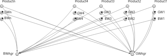
The water use by the agricultural sector accounts for the water footprint of agricultural products, which measures their water use per mass of produce, and adjusting the water use by including water losses and agricultural return flows. A separate sub-agent (AGR agent) is introduced to perform the calculations related to the agricultural sector to simplify the dynamic-system model (main model), and the required outputs (BWAgr, GWAgr) of the dynamic system model are called by the agent in the main model (see Figs. 3 and 4). The BWAgr is given by the expression within parentheses in Eq. (6).

$$AgrWD_t=\left(\sum_i\in ABW_i\times Product_i,t\right)\times \frac1E_Agr+OtherAgrWD$$

(6)

in which $AgrWD_t$ = the volume of agricultural water use during period t, $BW_i$ = blue water footprint of agricultural product i (cubic meters per ton), $Product_i,t$ = the amount of production of agricultural product i during period t (tons), $E_Agr$ = the overall irrigation efficiency, $OtherAgrWD$ = the volume of water consumed by agricultural products not included in the set A of agricultural products (in cubic meters). The set A includes those agricultural products with the largest yields and shares of the national food basket.

$$AgrReW_t=AgrWD_t\times AgrReCo$$

(7)

in which $AgrReW_t$ = the volume of water returned from agricultural water use during the period t, and $AgrReCo$ = the coefficient of water returned from agricultural water use.

$$IndDomReW_t=IndDomWD_t\times IndDomReCo$$

(8)

in which $IndDomReW_t$ = the volume of water returned from industrial and municipal water use during period t, and $IndDomReCo$ = the coefficient of water returned from industrial and municipal water uses.

$$ReSW_t=IndDomReSWCo\times IndDomReW_t+AgrReSWCo\times AgrReW_t$$

(9)

in which $ReSW_t$ = the volume of water returned from water uses to surface water resources during period t, $IndDomReSWCo$ = the percentage of water returned from municipal and industrial water use to surface water resources, and $AgrReSWCo$ = the percentage of water returned from agricultural water use to surface water resources.

Water is applied to produce energy, and Eqs. (10) through (15) perform the related calculations. The $WEIF_t$ variable in Eq. (14) is necessary to account for the volume of water saved as a result of the energy savings. A PR model is introduced to account for such water savings (see Fig. 3).

$$Diff_t =OutputE_t-OutputE_t^P$$

(10)

in which $Diff_t$= the difference between the energy used in the main model during period t and the energy used in period t in the PR model, $OutputE_t$ = the sum of energy uses during period t in the main model (the method of calculating $OutputE_t$ is described in detail in “Energy uses”), and $OutputE_t^P$ = the sum of energy uses during period t in the PR model. Equations (11) and (12) account for the case when energy use exceeds energy production under current conditions, in which case energy exports are reduced. This prevents additional energy production to meet excess demand, and, consequently, there would not be increases in water use.

$$Diff_t \le 0\,\,\,if\,\,func_t=0$$

(11)

$$Diff_t >0\,\,\, if\,\,func_t=Diff_t$$

(12)

in which $ iffunc_t$ = the amount of energy saved during period t.

Equation (13) calculates the water required to produce energy:

$$TotalWE_t=Coal_t\times ENwateruseC+Gas_t\times ENwateruseG+OilPetroleumP_t \times ENwateruseO+Nuclear_t\times ENwateruseN+Elec_t\times ENwateruseE$$

(13)

in which $TotalWE_t$ = the volume of water required to produce the energy demand during period t,$Elec_t$ = the amount of electricity production during period t (MWh), and $ENwateruseE$ = the water required per unit of energy generated by electricity (cubic meters per MWh), all other terms were previously defined.

Equation (14) calculates the water savings:

$$WEIF_t=\sum_t=1^T\fracTotalWE_tOutputE_t^0\times if\,\,func_t$$

(14)

in which $WEIF_t$= the volume of water saved as a result of the energy saved during period t, T = the number of periods of simulation (T = 5 years).

Part of the water used to produce energy from coal, oil, petroleum products, and nuclear fuel is accounted for in the industrial sector water use. For this reason, the volume of water to produce energy calculated with Eq. (15) is reduced by that part of water already accounted for in the industrial water use to avoid double accounting.

$$WE_t=Coal_t\times ENwateruseC+Gas_t\times ENwateruseG+OilPetroleumP_t \times ENwateruseO+Nuclear_t\times ENwateruseN-INDE\times IndWD_t-WEIF_t$$

(15)

in which $WE_t$ = the volume of water required to produce different types of energy (except those included in the industrial sector) during period t, $Coal_t$ = the energy produced with coal during period t (MWh), $ENwateruseC$ = the water required per unit of energy produced with coal (cubic meters per MWh),$Gas_t$ = the amount of energy produced with natural gas during period t (MWh), $ENwateruseG$ = the water required per unit of energy produced with natural gas (cubic meters per MWh), $OilPetroleumP_t$ = the amount of energy produced with crude oil and other petroleum products during period t (MWh), $ENwateruseO$ = the water required per unit of energy produced with crude oil and petroleum products (cubic meters per MWh),$Nuclear_t$ = the amount of nuclear energy produced during period t (MWh), $ENwateruseN$ = the water required per unit of nuclear energy produced (cubic meters per MWh), and $INDE$ = the percentage of industrial water use already accounted for in Eq. (5) (which pertains to water used in the coke coal, oil refineries, and nuclear fuel industries).

Part of the discharge of springs enters the surface water sources, and this enters the calculation of the input to the surface water-resources stock in Eq. (16):

$$InputSW_t= SInflow+ReSW_t+ Fountain_t$$

(16)

in which $InputSW_t$ = the volume of inflow water to surface water sources during period t, and $Fountain_t$ = discharge of springs to surface water sources during period t, other terms previously defined.

The output of the surface water resources includes water use and the infiltration of surface water into groundwater, the latter calculated with Eq. (17):

$$SInflowInf_t=SInflow_t\times SInflowInfCo$$

(17)

in which $SInflowInf_t$ = the infiltration volume of surface water during period t, and $SInflowInfCo$ = the infiltration coefficient of surface water.

The output of the surface water resources stock is calculated using Eq. (18):

$$OutputSW_t=AgrSWDCo_t\times AgrWD_t+IndSWDCo_t\times IndWD_t+DomSWDCo_t\times DomWD_t+\mathrm WE_t+SInflowInf_t-EvSwSea_t$$

(18)

in which $OutputSW_t$ = the output volume of surface water during period t, $AgrSWDCo_t$ = the percentage of gross agricultural water use from surface water resources during period t, $IndSWDCo_t$ = the percentage of industrial water use from surface water resources during period t, $DomSWDCo_t$= the percentage of gross drinking water consumption from surface water sources during period t, and $EvSwSea_t$ = the total volume of evaporation from surface water plus the discharge of surface water to the sea during period t.

The balance of surface water resources is calculated based on Eq. (19):

$$SWater\left(t\right)=\undersett_0\oversett\int \left[InputSW_t\left(S\right)-OutputSW_t(S)\right]dt+SWater(0)$$

(19)

in which $SWater\left(t\right)$ = the stock of surface water resources at time t, $SWater(0)$ denotes the stock of surface water at the initial time (t = 0).

Groundwater resources

Groundwater resources gain water from deep infiltration of precipitation in the plains and elevated areas from (1) inflows from outside of the study area, (2) infiltration from surface flows and return waters. Groundwater output factors also include the discharge of groundwater resources (wells, springs, and aqueducts), groundwater flow that moves outside the study area and evaporation. Infiltration of precipitation in the plains and in high terrain into groundwater resources is calculated with Eq. (20):

$$Inf_t=PrePInfCo\times preplain_t+PreHInfCo\times preheight_t$$

(20)

in which $Inf_t$ = the volume of water entering groundwater sources through infiltration of precipitation during period t, $PrePInfCo$ = the infiltration coefficient of precipitation in the plains, and $PreHInfCo$ = the infiltration coefficient of rainfall in high terrain.

Equation (21) calculates the volume of return water that accrues to groundwater resources:

$$ReGW_t=IndDomReGWCo\times IndDomReW_t+AgrReGWCo\times AgrReW_t$$

(21)

in which $ReGW_t$ = the volume of water returned from water use that accrues to groundwater resources during period t, $IndDomReGWCo$ = the percentage of water returned from municipal and industrial water use accruing to groundwater resources, and $AgrReGWCo$ = the percentage of water returned from agricultural water use accruing to groundwater resources.

The volume of groundwater input is calculated with Eq. (22):

$$InputGW_t=Inf_t+ReGW_t+SInflowInf_t+OutCGw _t$$

(22)

in which $InputGW_t$ = the volume of groundwater input during period t, and $OutCGw _t$ = the difference between the volume of groundwater leaving and that entering the country during period t.

The volume of groundwater output is calculated with Eq. (23):

$$OutputGW_t=AgrGWDCo_t\times AgrWD_t+IndGWDCo\times IndWD_t+DomGWDCo\times DomWD_t+EvGwDr_t$$

(23)

in which $OutputGW_t$ = the volume of groundwater output during period t, $AgrGWDCo_t$ = the percentage of gross agricultural water use from groundwater resources during period t, IndGWDCo = the percentage of industrial water use from groundwater resources during period t, DomGWDCo = the percentage of municipal water use from groundwater resources during period t, and $EvGwDr _t$ = the total volume of evaporation from groundwater plus the drainage of groundwater resources to surface water resources at time t.

Equation (24) calculates the annual balance of groundwater resources:

$$GWater\left(t\right)=\undersett_0\oversett\int \left[InputGW_t\left(S\right)-OutputGW_t\left(S\right)\right]dt+GWater(0)$$

(24)

in which GWater(t) = the groundwater resources stock at time t, $GWater(0)$ denotes the stock of groundwater at the initial time (t = 0).

Energy uses

Energy uses are calculated with Eqs. (25)–(27). The total national energy use includes the agricultural, industrial, transportation, and exports sectors’ energy demands. The energy uses by these sectors do not change during the implementation of the policy, and, consequently do not change the WFE Nexus in that period; therefore, they are not included in the calculations.

$$WDTP_t=DomWD_t\times CEIntensity_t$$

(25)

in which $WDTP_t$ = the energy used in the extraction, transmission, distribution, and treatment of water in the water and wastewater system during period t, and $CEIntensity_t$ = the energy intensity in the extraction, transmission, distribution, and treatment of water in water and wastewater systems during the period t (MWh per cubic meter).

$$ResComPubED_t=ResComPubPerCapita\times Population_t$$

(26)

in which $ResComPubED_t$ = the energy use by the domestic, commercial, and public sectors during period t, and $ResComPubPerCapita$ = the per capita energy consumption by the domestic, commercial, and public sectors (MWh per person per year).

$$OutputE_t=ResComPubED_t+WDTP_t$$

(27)

Environmental water needs

The gray water footprint is defined as the volume of freshwater that is required to assimilate the load of pollutants based on natural background concentrations and existing ambient water quality standards. The estimation of the gray water footprint associated with discharges from agricultural production is based on the load of nitrogen fertilizers, which are pervasive in agriculture. The gray water footprint in terms of nitrogen concentration has been estimated by Mekonnen and Hoekstra^24,25, as written in Eq. (28):

$$GW_t^Agr=\sum_i\in AGW_i\times Product_i,t$$

(28)

in which $GW_t^Agr$= the volume of gray water in the agricultural sector during period t, and $GW_i$ = the volume of gray water associated with the production of one ton of agricultural product i (cubic meters per ton)$.$

There are no accurate estimates of the concentrations of pollutants per unit of industrial production, or of the concentration of pollutants in municipal wastewater. Therefore, the conservative dilution factor (DF), which is equal to 1 for untreated returned water from the municipal and industrial sectors, is applied in this work. Equation (29) is a simplified equation of the gray water footprint²⁶. The fraction appearing on the right-hand side of Eq. (29) is equal to the DF.

$$GW_t^IndDom= \fracC_eff-C_natC_max-C_nat\times IndDomReW_t\times IndDomReUT$$

(29)

in which $GW_t^IndDom$ = the gray water footprint of the municipal and industrial sectors during period t, $C_eff$ = the nitrogen concentration in return water (mg/L), $C_nat$ = the natural concentrations of contaminant in surface water (mg/L), $C_max$ = the maximum allowable concentration contaminant in surface water (mg/L), and $IndDomReUT$ = the percentage of untreated returned water from the municipal and industrial sectors.

The total gray water footprint is obtained by summing the footprints associated with the municipal/industrial and agricultural sectors:

$$TotalGW_\mathrmt=GW_t^IndDom+GW_t^Agr$$

(30)

in which $TotalGW_\mathrmt$ = the volume of gray water from all sectors during period t.

This work considers qualitative and quantitative environmental water needs. Equation (31) is used to calculate the total environmental water need. The Tennant method for calculating the riverine environmental flow requirement (or instream flow) stipulates that, based on the conditions of each basin, between 10 to 30% of the average long-term flow of rivers represents the environmental flow requirement²⁷. The sum of these requirements across all the basins equals the environmental requirement of the entire region or country. Yet, by providing 10 to 30% of the average long-term flow of rivers the riverine ecosystem barely emerges from critical conditions, and is far from optimal ecologic functioning. The total environmental water need is equal to the sum of the environmental flow requirement plus the volume of water needed to dilute the contaminants entering the surface water sources:

$$ENV_t=TotalGW_t+Tennant$$

(31)

in which $ENV_t$ = the environmental flow requirement during period t, and Tennant = the environmental flow requirement calculated by the Tennant (1976) method.

The policy evaluation index

The available renewable water is calculated with Eq. (32):

$$IN_t=OutCGW _t+ SInflow _t+ Inf_t-EvGwDr_t$$

(32)

in which $IN_t$= the renewable water available before the application of environmental constraints during period t.

The volume of manageable water is calculated with Eq. (33):

$$REW\left(t\right)=\undersett_0\oversett\int \left[IN\left(t\right)-ENV\left(t\right)\right]dt$$

(33)

in which REW (t) = the (cumulative) manageable and exploitable renewable water in the period t-t₀.

Equation (34) calculates the total water withdrawals by the agricultural, industrial, municipal, and energy production sectors:

$$WDW_t=OutputSW _t+ OutputGW_t- cheshmeh_t$$

(34)

in which $WDW_t$ = the sum of the withdrawals by the agricultural, industrial, municipal, and energy production sectors during period t.

The cumulative water withdrawals are calculated with Eq. (35):

$$withd\left(t\right)=\undersett_0\oversett\int WDW\left(t\right)dt$$

(35)

in which $withd\left(t\right)$ = the sum of the withdrawals by the agricultural, industrial, municipal and energy production sectors in the horizon t-t₀.

Equation (36) calculates the water stress index:

$$index_t_f^MRW=\fracwithd(t_f)REW\left(t_f\right)\times 100$$

(36)

in which $index_t_f^MRW$ = the renewable water stress index at the end of the study period, and $t_f$ = the period marking the end of the study horizon.

Once the water and energy model is developed it must be calibrated with observational data prior to its use in predictions, as shown below.